Estimating polymer consumption accurately is essential for budget planning, procurement scheduling, and treatment system design. Whether you are designing a new treatment system, evaluating a process change, or simply trying to forecast annual chemical spend, a reliable consumption estimate prevents both the operational disruption of running short and the capital waste of overstocking.
Three methods are available for estimating PAM consumption, each appropriate for different situations: theoretical calculation from wastewater characteristics, jar testing on representative samples, and benchmarking against comparable facilities. The most reliable estimates combine all three approaches — using theory to establish a starting range, jar testing to refine it, and benchmarks to validate the result.
Method 1: Theoretical Calculation
Theoretical consumption estimation works from first principles — the mass of suspended solids requiring treatment and the polymer-to-solids ratio needed to achieve target treatment performance.
Step 1: Determine Suspended Solids Loading
TSS loading (kg/day) = Influent flow (m³/day) × TSS concentration (mg/L) ÷ 1,000
Example:
- Flow: 2,000 m³/day
- TSS: 3,000 mg/L
- TSS loading = 2,000 × 3,000 ÷ 1,000 = 6,000 kg/day
Step 2: Apply Polymer-to-Solids Ratio
The polymer-to-solids ratio (also called specific polymer demand) is the mass of PAM required per unit mass of dry solids treated. This ratio varies significantly by application:
| Application | Typical Polymer:Solids Ratio | Notes |
|---|---|---|
| Mineral processing thickener | 50–200 g/tonne DS | High MW anionic PAM |
| Coal washing thickener | 100–300 g/tonne DS | High MW anionic PAM |
| Municipal primary clarifier | 0.5–2 g/tonne DS | Low-dose application |
| Municipal sludge dewatering | 3,000–8,000 g/tonne DS | Cationic PAM, dewatering |
| Industrial clarifier (moderate SS) | 200–800 g/tonne DS | Application-specific |
| Sand/gravel settling pond | 100–400 g/tonne DS | High MW anionic PAM |
Estimated PAM consumption (kg/day) = TSS loading (kg/day) × Polymer:Solids ratio (g/kg) ÷ 1,000
Example (mineral processing thickener):
- TSS loading: 6,000 kg/day
- Polymer:Solids ratio: 120 g/tonne = 0.12 g/kg
- PAM consumption = 6,000 × 0.12 ÷ 1,000 = 0.72 kg/day…
(Correction: 6,000 kg/day at 120 g/tonne = 6,000 × 120/1,000,000 tonnes × 1,000 = 720 g/day = 0.72 kg/day)
More practically expressed: 120 g/tonne × 6 tonnes/day = 720 g/day = 0.72 kg/day
Step 3: Convert to Volumetric Dosage for Verification
Cross-check the theoretical consumption against a dosage expressed in mg/L:
Dosage (mg/L) = PAM consumption (kg/day) ÷ Flow (m³/day) × 1,000
Example: 0.72 kg/day ÷ 2,000 m³/day × 1,000 = 0.36 mg/L
For a mineral processing thickener at moderate SS concentration, 0.36 mg/L is on the low end of typical — suggesting the polymer:solids ratio should be checked against more specific data for the ore type. This cross-check is the value of the theoretical approach: it identifies when estimates appear outside realistic ranges before a procurement commitment is made.
Request product specifications and pricing to support your consumption estimate and procurement planning. → Get in touch today
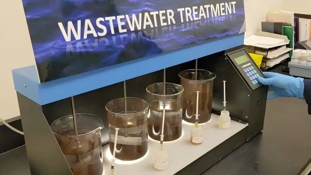
Method 2: Jar Testing
Jar testing provides the most reliable consumption estimate for a specific wastewater at specific conditions. It directly measures the dosage required to achieve target treatment performance — without the uncertainty of generic polymer:solids ratios.
Jar Test Consumption Estimation Procedure
Step 1: Collect a representative wastewater sample from the actual treatment point.
Step 2: Prepare PAM solution at 0.1% concentration (1 g/L).
Step 3: Test dosages spanning a range around the expected optimum — typically 5–7 dosage levels.
Step 4: For each dosage, evaluate floc formation, settling rate, and supernatant clarity. Identify the minimum dosage achieving target performance — this is the optimal dose.
Step 5: Convert optimal dose to consumption:
Daily consumption (kg/day) = Optimal dose (mg/L) × Flow (m³/day) ÷ 1,000
Example:
- Optimal dose from jar test: 4 mg/L
- Flow: 5,000 m³/day
- Daily consumption = 4 × 5,000 ÷ 1,000 = 20 kg/day
- Annual consumption = 20 × 365 = 7,300 kg/year = 7.3 tonnes/year
Jar Test Limitations for Consumption Estimation
Jar testing provides the most accurate estimate of dosage under the specific conditions of the test — but real-world consumption will vary around this point due to:
- Influent variability (different solids concentrations, particle types, seasonal changes)
- Temperature effects on polymer performance
- Dosage management quality (consistent dosing vs. reactive adjustment)
- Product quality variation between batches
Apply a real-world variability factor of 15–25% above the jar test optimum for annual budget purposes — this accounts for the higher dosages applied during adverse conditions while the jar test represents best-case optimum conditions.
Budget consumption estimate = Jar test optimal dose × 1.15 to 1.25
Method 3: Industry Benchmarks
Benchmark data from similar facilities provides a sanity check on theoretical calculations and jar test results, and is particularly useful for new installations where site-specific data is not yet available.
Consumption Benchmarks by Application
Municipal wastewater treatment (combined clarification and dewatering):
- Typical range: 0.5–2.0 kg active PAM per 1,000 m³ treated
- Specific consumption above 2.5 kg/1,000 m³ suggests either high-solids influent or an underoptimized polymer program
Mining mineral processing thickeners:
- Typical range: 50–200 g active PAM per tonne of dry ore processed
- Highly variable by ore type — iron ore at the low end, clay-rich ores at the high end
Sand and gravel washing:
- Typical range: 0.8–3.0 kg/1,000 m³ process water
- Higher end for operations with high clay content or fine particle fraction
Industrial sludge dewatering (belt press):
- Typical range: 3–8 kg cationic PAM per tonne of dry solids dewatered
- Higher for biological sludge, lower for mineral sludge
Coal washing:
- Typical range: 100–300 g/tonne of coal processed
Using Benchmarks Correctly
Benchmarks provide a validity range — not a target. If your estimate falls within the benchmark range, it is plausible. If it falls outside, investigate the reason before accepting the estimate.
Common reasons for above-benchmark consumption:
- Higher-than-average solids concentration
- Clay-rich or fine-particle-dominant influent
- Suboptimal polymer grade for the application
- Poor preparation quality reducing active polymer delivery
- Conservative dosage management
Common reasons for below-benchmark consumption:
- Cleaner-than-average influent
- Highly optimized program with automated dosage control
- Higher MW grade than the benchmark assumption
Combining All Three Methods: A Practical Approach
For new facility design or major process changes, use all three methods in sequence:
Phase 1 — Scoping (Theory): Use theoretical calculation to establish order-of-magnitude consumption. This determines procurement scale and budget range before any testing is possible.
Phase 2 — Optimization (Jar Testing): Conduct jar testing with representative samples as soon as they are available. Refine the estimate to a specific dosage at defined conditions.
Phase 3 — Validation (Benchmarks): Compare jar test-derived consumption against industry benchmarks. Investigate and resolve significant discrepancies before finalizing the estimate.
Phase 4 — Budget Adjustment: Apply the 15–25% variability factor to the jar test optimum for budget purposes. Build a seasonal adjustment if significant temperature variation is expected.
Frequently Asked Questions
How do we estimate consumption for a facility not yet built?
Use theoretical calculation from design influent specifications combined with benchmark data for the intended application type. Apply a conservative variability factor of 25–30% above the theoretical estimate for budget purposes — actual consumption will be confirmed during commissioning jar testing. Request indicative pricing from suppliers based on your estimated range before design is finalized.
Our actual consumption is consistently 30% above our jar test estimate — why?
The most common causes are: influent variability requiring higher dosage during adverse periods that the jar test did not capture; preparation quality issues reducing active polymer delivery (fish eyes, incomplete hydration); conservative dosage management adding margin above the true optimum; and batch-to-batch product quality variation. Review each cause systematically — the 30% gap often has a single dominant explanation that, once addressed, brings consumption back toward the jar test estimate.
How often should we re-estimate consumption after initial optimization?
Re-estimate when any significant change occurs: production rate change above 20%, new raw material source, seasonal transition with significant temperature change, supplier or grade change. For stable operations, an annual consumption review comparing actual against estimated provides adequate oversight without excessive testing burden.
Conclusion
Accurate PAM consumption estimation combines theoretical calculation, jar testing, and benchmark validation into a layered approach that is more reliable than any single method alone. Theoretical calculation provides the starting framework; jar testing grounds it in site-specific reality; benchmarks validate the result against comparable operations.
For budget planning, the jar test optimum adjusted by a 15–25% variability factor is the most practical and defensible estimate. For facility design, conservative theoretical estimates validated by pilot-scale testing before final design commitment is the standard approach.
Contact our technical team today to request jar testing support, grade recommendations, and consumption estimates for your specific application. → Contact our technical team today