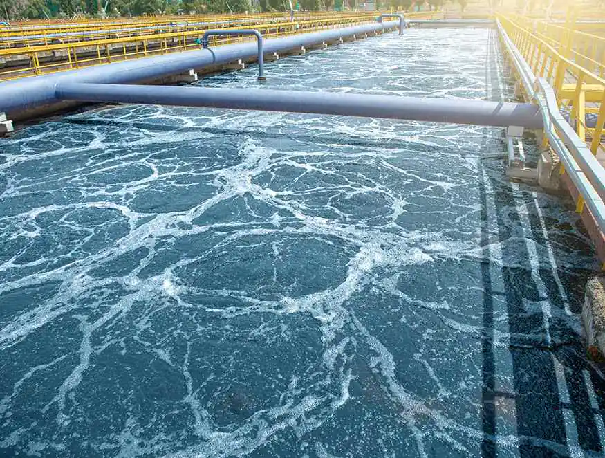
Mixing energy is one of the most technically important — and most frequently overlooked — variables in PAM-assisted flocculation. Too little mixing, and polymer cannot distribute effectively through the wastewater stream. Too much mixing, and the flocs being built are simultaneously destroyed. Between these extremes lies an optimal range that varies by treatment stage and application — and getting it right determines how much of the polymer’s rated flocculation capacity is actually delivered to the treatment system.
For engineers designing new treatment systems or diagnosing underperforming existing ones, understanding mixing energy quantitatively — through the velocity gradient G and its time integral Gt — provides the analytical framework for systematic optimization rather than trial-and-error adjustment.
The Velocity Gradient (G Value): The Key Parameter
Mixing intensity in flocculation systems is characterized by the velocity gradient G, expressed in units of reciprocal seconds (s⁻¹). G represents the rate of fluid shear in the mixing zone — higher G means more intense mixing.
G is calculated from:
G = √(P / (μ × V))
Where:
- G = velocity gradient (s⁻¹)
- P = power input to the fluid (W)
- μ = dynamic viscosity of the fluid (Pa·s)
- V = volume of the mixing zone (m³)
For water at 20°C: μ = 1.002 × 10⁻³ Pa·s For water at 10°C: μ = 1.307 × 10⁻³ Pa·s
This temperature dependence matters: the same agitator at the same speed produces lower G in cold water than in warm water — a contributing factor to winter performance decline that is often overlooked in seasonal troubleshooting.
G Values for Each Stage of PAM-Assisted Treatment
Different stages of the coagulation-flocculation process require different G values. Applying the wrong mixing intensity at any stage reduces overall treatment efficiency.
Stage 1: Coagulant Rapid Mix
Recommended G: 200–1,000 s⁻¹ Residence time: 30–120 seconds
High G ensures coagulant contacts all particles before precipitation reactions are complete. G below 100 s⁻¹ in rapid mix allows coagulant to react with only a fraction of particles, producing uneven charge neutralization and poor subsequent flocculation.
Stage 2: PAM Addition and Initial Distribution
Recommended G: 100–300 s⁻¹ Residence time: 30–60 seconds
PAM should be introduced into a zone with sufficient turbulence to distribute the polymer rapidly but not so much shear that polymer chains are degraded before adsorbing onto particles. Many facilities add PAM at the same point as coagulant (G too high) or directly into the flocculation chamber (G too low) — both reduce performance.
Request technical consultation and product specifications for your flocculation system optimization. → Get in touch today
Stage 3: Slow Flocculation
Recommended G: 10–80 s⁻¹, tapering from high to low Residence time: 10–30 minutes
This is the stage where most floc growth occurs. Progressively decreasing G — called tapered flocculation — produces larger, more robust flocs than fixed mixing intensity throughout. Each G reduction allows slightly larger flocs to survive while still maintaining enough turbulence for particle collisions.
Stage 4: Transfer to Settling Zone
Recommended G: Below 10 s⁻¹
The flow path from flocculation zone to clarifier inlet should impose minimum shear. Pumps, sharp bends, and constrictions break flocs grown carefully in the flocculation stage.
The Gt Parameter: Combining Intensity and Time
G alone characterizes mixing intensity at a single point. Gt — the product of G and hydraulic residence time t — characterizes total mixing energy over the complete flocculation stage.
Gt = G × t (t in seconds)
| Application | Recommended Gt Range |
|---|---|
| High-turbidity industrial wastewater | 30,000–150,000 |
| Low-turbidity municipal wastewater | 20,000–100,000 |
| PAM-assisted flocculation (typical) | 15,000–80,000 |
| Sand and gravel washing | 20,000–60,000 |
Lower Gt is typically needed with PAM than without coagulant-only systems — polymer bridging accelerates floc formation, reducing the residence time needed for target performance.
Calculating G for Common Equipment Types
Mechanical Agitators
P = Np × ρ × n³ × D⁵
Where:
- Np = impeller power number (0.3–5.0 depending on type)
- ρ = fluid density ≈ 1,000 kg/m³
- n = rotational speed (rev/s)
- D = impeller diameter (m)
Then: G = √(P / (μ × V))
Worked example:
- Rushton turbine: Np = 5.0, n = 1.0 rev/s (60 RPM), D = 0.3 m, V = 2 m³, μ = 1.002 × 10⁻³ Pa·s
P = 5.0 × 1,000 × 1.0³ × 0.3⁵ = 12.15 W
G = √(12.15 / (1.002 × 10⁻³ × 2)) = √(6,063) = 77.9 s⁻¹
This places the agitator in the appropriate range for slow flocculation.
Hydraulic Mixing in Pipes
For inline static mixers or pipe constrictions used for rapid chemical addition:
G = √(ρ × g × hL / (μ × t))
Where hL = head loss across the mixing zone (m), t = hydraulic residence time (s).
This formula applies to PAM addition via static mixer — useful for characterizing G in pipe injection systems without mechanical agitation.

Designing a New Flocculation System: Worked Example
For a PAM-assisted system treating 5,000 m³/day (0.0579 m³/s):
Step 1 — Set target Gt: For moderately turbid industrial wastewater with PAM: Gt = 40,000
Step 2 — Select G, solve for t: At G = 30 s⁻¹: t = 40,000 / 30 = 1,333 seconds = 22 minutes
Step 3 — Calculate tank volume: V = Q × t = 0.0579 × 1,333 = 77 m³
Step 4 — Design tapered zones:
| Zone | G (s⁻¹) | Volume (m³) | Purpose |
|---|---|---|---|
| Zone 1 | 60 | 20 | Rapid initial floc growth |
| Zone 2 | 30 | 30 | Moderate floc development |
| Zone 3 | 15 | 27 | Gentle conditioning before clarifier |
Tapered flocculation consistently produces larger, more stable flocs than a single fixed G across the full tank volume.
Diagnosing Mixing Problems in Existing Systems
G value analysis frequently reveals the root cause of underperformance in existing systems. Common problems identified through G calculation:
Rapid mix G below 200 s⁻¹: Coagulant not distributing adequately — relocate dosing to higher-shear zone (pump discharge, in-pipe constriction).
PAM addition at G above 500 s⁻¹: Polymer chains degraded before adsorption — move PAM dosing point downstream to moderate-shear zone.
Fixed flocculation G throughout: No taper — add baffles or reduce agitator speed in later zones for larger floc production.
G above 5 s⁻¹ in transfer line to clarifier: Shear breaking flocs in transport — reduce flow velocity, eliminate constrictions, or relocate PAM dosing closer to clarifier.
For guidance on dosing point optimization in clarifier systems, see: Integrating PAM in Clarifier Systems Effectively
Temperature Correction for G Values
Because water viscosity increases at lower temperatures, the same agitator produces lower G in winter than in summer.
G_cold = G_warm × √(μ_warm / μ_cold)
Example: G = 50 s⁻¹ at 20°C → G at 5°C:
- μ at 20°C = 1.002 × 10⁻³ Pa·s
- μ at 5°C = 1.519 × 10⁻³ Pa·s
- G at 5°C = 50 × √(1.002/1.519) = 50 × 0.812 = 40.6 s⁻¹
An 18% reduction in effective G — the system is operating outside its designed mixing intensity range. For cold-climate facilities, increasing agitator RPM in winter to restore target G partially compensates for this effect alongside other winter adjustments.
Frequently Asked Questions
How do I measure G in an existing tank without detailed equipment data?
Measure power draw at the agitator motor using a clamp meter, then calculate G directly from P, μ, and V. Allow for motor and gearbox efficiency losses — typically 85–90% of motor input reaches the fluid. For a more detailed characterization, tracer studies can map residence time distribution and effective G within the tank.
What G should I use for inline PAM dosing into a pipe without a static mixer?
For pipe injection without a static mixer, G is determined by flow velocity and friction. At typical industrial pipe velocities, G ranges from 100–500 s⁻¹ — often higher than ideal for PAM addition. Adding a short static mixer with a controlled pressure drop provides a defined, appropriate G zone for polymer distribution without requiring a separate mixing tank.
Does G value optimization differ for anionic versus cationic PAM?
The principles are the same, but cationic grades used in sludge dewatering are less sensitive to G management than anionic clarification grades — dewatering equipment provides its own mixing action, and contact time is typically more important than G precision in dewatering applications.
Conclusion
Mixing energy — characterized through velocity gradient G and the integrated parameter Gt — provides the engineering framework for designing and optimizing PAM flocculation systems. Each treatment stage has a defined optimal G range: high for rapid coagulant distribution, moderate for PAM addition, progressively tapering through slow flocculation, and minimal in transfer to the settling zone.
Applying G value analysis to underperforming systems frequently identifies the mixing-related root cause of performance problems that dosage and grade changes alone cannot resolve. For new system design, the calculation framework in this guide provides the basis for sizing flocculation tanks and specifying tapered mixing zones that maximize PAM performance.
Contact our technical team today for PAM grade recommendations and application support that complement your mixing system design. → Contact our technical team today